Tutorial & Visualisation

Get the data

Import the module:

import H5CosmoKit as ckit

You can download e.g. snapshot_090 (z = 0.00) directly within this notebook.

urls = ["https://users.flatironinstitute.org/~camels/Sims/IllustrisTNG/CV/CV_0/snapshot_090.hdf5"] # extend the list as needed
local_files = ["snapshot_090.hdf5"]

for url, local_file in zip(urls, local_files):
    ckit.download_file(url, local_file)

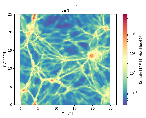
Density & Temperature

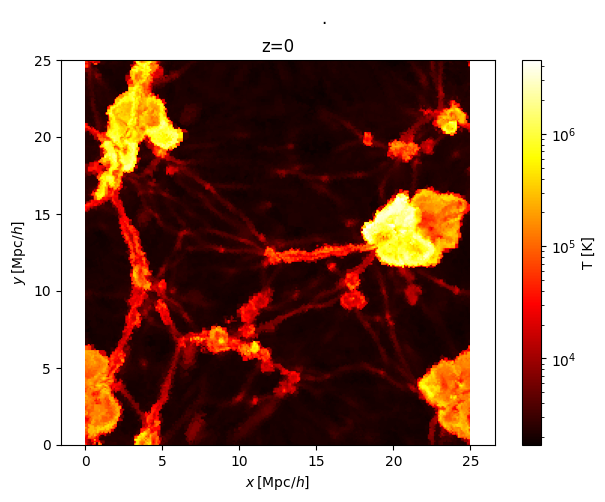
Now that we have the data, we can use the H5CosmoKit package to visualize density and temperature simple with preview().

path = '.'  # Path to the snaps
snapshot_numbers = [90] # list of desired snapfile numbers

ckit.preview(path, snapshot_numbers, 'gas_density')
ckit.preview(path, snapshot_numbers, 'gas_temperature')

For interactive 3D visualization, you can use the preview_3d() function.

subset_size = 300000
ckit.preview_3d(path, snapshot_numbers, 'gas_density', subset_size)

- [View the 3D Density Plot](_static/Snapshot_90_at_z=0.00_gas_density.html)

subset_size = 150000
ckit.preview_3d(path, snapshot_numbers, 'gas_temperature', subset_size)

• View the 3D Temperature Plot

Soundspeed & Internal Energy

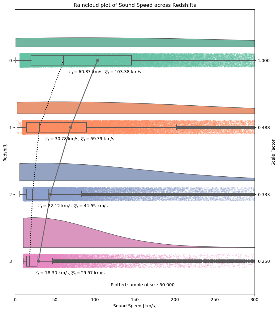
You can visualize the distribution of sound speed or internal energy as a raincloud plot.

ckit.plot_internalenergy_distribution(
    path='/gpfs/data/fs72085/mfo/CAMELS/CV0',
    snapshot_numbers=[32, 44, 60, 90],
    sample_size=50000
)

In addition to visualizing these distributions, you can also fit a polynomial to the median values of the sound speed or internal energy across multiple snapshots using the functions plot_median_soundspeed_with_polynomial_fit() and plot_median_internalenergy_with_polynomial_fit().

ckit.plot_median_internalenergy_with_polynomial_fit(path, snapshot_numbers)

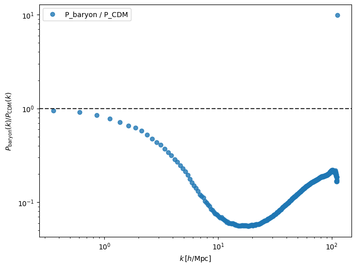
Power Spectra

As power spectra analysis uses Pylians, you might experience difficulties on machines other than Linux and Mac. For more details, visit the Pylians documentation.

f_snap = './snapshot_090.hdf5'
ckit.power_ratio(f_snap)

Using CIC mass assignment scheme with weights
Time taken = 1.498 seconds


Computing power spectrum of the field...

Time to complete loop = 6.31
Time taken = 9.80 seconds

Using CIC mass assignment scheme with weights

Time taken = 1.285 seconds


Computing power spectrum of the field...

Time to complete loop = 6.29
Time taken = 9.20 seconds

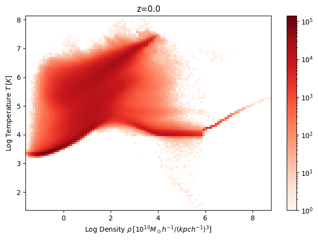
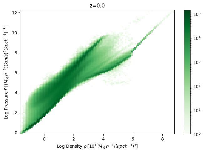
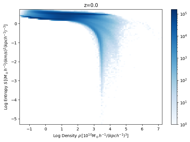
Phase diagrams

ckit.preview_phase_diagram(path, snapshot_numbers, quantity='temperature')
ckit.preview_phase_diagram(path, snapshot_numbers, quantity='pressure')
ckit.preview_phase_diagram(path, snapshot_numbers, quantity='entropy')